Hash table

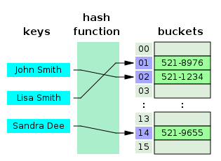
 In computing, a hash table (hash map) is a data structure that implements an associative array abstract data type, a structure that can map keys to values. A hash table uses a hash function to compute an index, also called a hash code, into an array of buckets or slots, from which the desired value can be found. During lookup, the key is hashed and the resulting hash indicates where the corresponding value is stored.

Hash table
Type	Unordered associative array
Invented	1953
Time complexity in big O notation
Algorithm Average Worst case Space O(n)[1] O(n) Search O(1) O(n) Insert O(1) O(n) Delete O(1) O(n)

A small phone book as a hash table

Ideally, the hash function will assign each key to a unique bucket, but most hash table designs employ an imperfect hash function, which might cause hash collisions where the hash function generates the same index for more than one key. Such collisions are typically accommodated in some way.

In a well-dimensioned hash table, the average cost (number of instructions) for each lookup is independent of the number of elements stored in the table. Many hash table designs also allow arbitrary insertions and deletions of key–value pairs, at (amortized^[2]) constant average cost per operation.^[3][4]

In many situations, hash tables turn out to be on average more efficient than search trees or any other table lookup structure. For this reason, they are widely used in many kinds of computer software, particularly for associative arrays, database indexing, caches, and sets.

HashingEdit

Main article: Hash function

The advantage of using hashing is that the table address of a record can be directly computed from the key. Hashing implies a function ${\displaystyle h}$, when applied to a key ${\displaystyle k}$, produces a hash ${\displaystyle M}$. However, since ${\displaystyle M}$ could be potentially large, the hash result should be mapped to finite entries in the hash table—or slots—several methods can be used to map the keys into the size of hash table ${\displaystyle N}$. The most common method is the division method, in which modular arithmetic is used in computing the slot.^[5]: 110

${\displaystyle h(k)\ =\ M\ \operatorname {mod} \ N}$

This is often done in two steps,

${\displaystyle {\text{Hash}}={\text{Hash-Function(Key)}}}$

${\displaystyle {\text{Index}}={\text{Hash}}\ \%\ {\text{Hash-Table-Size}}}$

Choosing a hash functionEdit

A basic requirement is that the function should provide a uniform distribution of hash values. A non-uniform distribution increases the number of collisions and the cost of resolving them. Uniformity is sometimes difficult to ensure by design, but may be evaluated empirically using statistical tests, e.g., a Pearson's chi-squared test for discrete uniform distributions.^[6][7]

The distribution needs to be uniform only for table sizes that occur in the application. In particular, if one uses dynamic resizing with exact doubling and halving of the table size, then the hash function needs to be uniform only when the size is a power of two. Here the index can be computed as some range of bits of the hash function. On the other hand, some hashing algorithms prefer to have the size be a prime number.^[8] The modulus operation may provide some additional mixing; this is especially useful with a poor hash function.

For open addressing schemes, the hash function should also avoid clustering, the mapping of two or more keys to consecutive slots. Such clustering may cause the lookup cost to skyrocket, even if the load factor is low and collisions are infrequent. The popular multiplicative hash^[3] is claimed to have particularly poor clustering behavior.^[8]

Cryptographic hash functions are believed to provide good hash functions for any table size, either by modulo reduction or by bit masking. They may also be appropriate if there is a risk of malicious users trying to sabotage a network service by submitting requests designed to generate a large number of collisions in the server's hash tables. However, the risk of sabotage can also be avoided by cheaper methods (such as applying a secret salt to the data). A drawback of cryptographic hashing functions is that they are often slower to compute, which means that in cases where the uniformity for any size is not necessary, a non-cryptographic hashing function might be preferable.^{[citation needed]}

K-independent hashing offers a way to prove a certain hash function doesn't have bad keysets for a given type of hashtable. A number of such results are known for collision resolution schemes such as linear probing and cuckoo hashing. Since K-independence can prove a hash function works, one can then focus on finding the fastest possible such hash function.

Universal hash function is an approach of choosing a hash function randomly in a way that the hash function is independent of the keys that are to be hashed by the function. The possibility of collision between two distinct keys from a set is no more than ${\displaystyle 1/m}$ where ${\displaystyle m}$ is cardinality.^[9]: 264

Perfect hash functionEdit

Main article: Perfect hash function

If all keys are known ahead of time, a perfect hash function can be used to create a perfect hash table that has no collisions.^[10] If minimal perfect hashing is used, every location in the hash table can be used as well.^[11]

Perfect hashing allows for constant time lookups in all cases. This is in contrast to most chaining and open addressing methods, where the time for lookup is low on average, but may be very large, O(n), for instance when all the keys hash to a few values.

Key statisticsEdit

A critical statistic for a hash table is the load factor, defined as

${\displaystyle {\text{load factor}}\ (\alpha )={\frac {n}{k}}}$,

where

• ${\displaystyle n}$ is the number of entries occupied in the hash table.
• ${\displaystyle k}$ is the number of buckets.

The performance of the hash table worsens in relation to the load factor (${\displaystyle \alpha }$) i.e. as ${\displaystyle \alpha }$ approaches 1. Hence, it's essential to resize—or "rehash"—the hash table when the load factor exceeds an ideal value. It's also efficient to resize the hash table if the size is smaller—which is usually done when load factor drops below ${\displaystyle \alpha _{max}/4}$.^[12] Generally, a load factor of 0.6 and 0.75 is an acceptable figure.^{[13][5]: 110}

Collision resolutionEdit

See also: 2-choice hashing

The search algorithm that uses hashing consists of two parts. The first part is computing a hash function which transforms the search key into an array index. The ideal case is such that no two search keys hashes to the same array index, however, this is not always the case, since it's theoretically impossible.^[14]: 515 Hence the second part of the algorithm is collision resolution. The two common methods for collision resolution are separate chaining and open addressing.^[15]: 458

Separate chainingEdit

Hash collision resolved by separate chaining

Hash collision by separate chaining with head records in the bucket array.

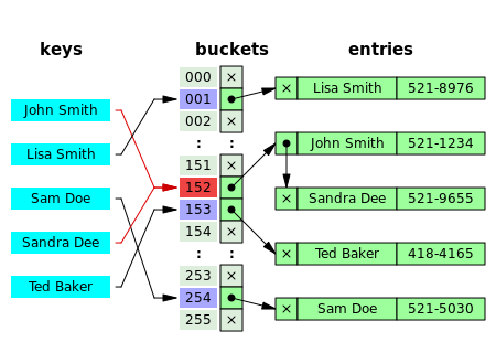
Hashing is an example of space-time tradeoff. If there exists a condition where the memory is infinite, single memory access using the key as an index in a (potentially huge) array would retrieve the value—which also implies possible key values are huge. On the other hand, if time is infinite, the values can be stored in minimum possible memory and a linear search through the array can be used to retrieve the element.^[15]: 458 In separate chaining, the process involves building a linked list with key-value pair for each search array indices. The collided items are chained together through a single linked list, which can be traversed to access the item with a unique search key.^[15]: 464 Collision resolution through chaining i.e. with a linked list is a common method of implementation. Let ${\displaystyle T}$ and ${\displaystyle x}$ be the hash table and the node respectively, the operation involves as follows:^[9]: 258

Chained-Hash-Insert(T, x) insert ${\displaystyle x}$ at the head of linked list ${\displaystyle T[h(x.key)]}$ Chained-Hash-Search(T, k) search for an element with key ${\displaystyle k}$ in linked list ${\displaystyle T[h(k)]}$ Chained-Hash-Delete(T, x) delete ${\displaystyle x}$ from the linked list ${\displaystyle T[h(x.key)]}$

If the keys of the elements are ordered, it's efficient to insert the item by maintaining the order when the key is comparable either numerically or lexically, thus resulting in faster insertions and unsuccessful searches.^{[14]: 520-521} However, the standard method of using a linked list is not cache-conscious since there is little spatial locality—locality of reference—since the nodes of the list are scattered across the memory, hence doesn't make efficient use of CPU cache.^[16]: 91

Separate chaining with other structuresEdit

If the keys are ordered, it could be efficient to use "self-organizing" concepts such as using a self-balancing binary search tree, through which the theoretical worse case could be bought down to ${\displaystyle O(\log {n})}$, although it introduces additional complexities.^[14]: 521

In cache-conscious variants, a dynamic array found to be more cache-friendly is used in the place where a linked list or self-balancing binary search trees is usually deployed for collision resolution through separate chaining, since the contiguous allocation patten of the array could be exploited by hardware-cache prefetchers—such as translation lookaside buffer—resulting in reduced access time and memory consumption.^[17][18][19]

In dynamic perfect hashing, two level hash tables are used to reduce the look-up complexity to be a guaranteed ${\displaystyle O(1)}$ in the worse case. In this technique, the buckets of ${\displaystyle k}$ entries are organized as perfect hash tables with ${\displaystyle k^{2}}$ slots providing constant worst-case lookup time, and low amortized time for insertion.^[20] A study shows array based separate chaining to be 97% more performant when compared to the standard linked list method under heavy load.^[16]: 99

Techniques such as using fusion tree for each buckets also result in constant time for all operations with high probability.^[21]

Open addressingEdit

Main article: Open addressing

Hash collision resolved by open addressing with linear probing (interval=1). Note that "Ted Baker" has a unique hash, but nevertheless collided with "Sandra Dee", that had previously collided with "John Smith".

This graph compares the average number of CPU cache misses required to look up elements in large hash tables (far exceeding size of the cache) with chaining and linear probing. Linear probing performs better due to better locality of reference, though as the table gets full, its performance degrades drastically.

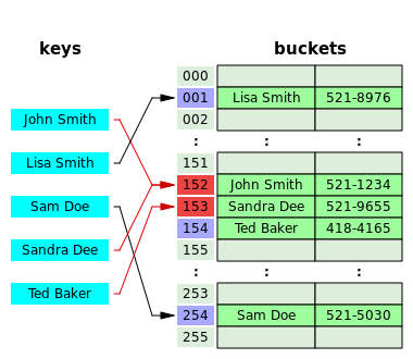
In another strategy, called open addressing, all entry records are stored in the bucket array itself. When a new entry has to be inserted, the buckets are examined, starting with the hashed-to slot and proceeding in some probe sequence, until an unoccupied slot is found. When searching for an entry, the buckets are scanned in the same sequence, until either the target record is found, or an unused array slot is found, which indicates that there is no such key in the table.^[22] The name "open addressing" refers to the location ("address") of the item is not determined by its hash value. (This method is also called closed hashing; it should not be confused with "open hashing" or "closed addressing" which usually means separate chaining.)

Well-known probe sequences include:

• Linear probing, in which the interval between probes is fixed (usually 1). Since the slots are located in successive locations, linear probing could lead to better utilization of CPU cache due to locality of references.^[23]
• Quadratic probing, in which the interval between probes is increased by adding the successive outputs of a quadratic polynomial to the starting value given by the original hash computation
• Double hashing, in which the interval between probes is computed by a second hash function

In practice, the performance of open addressing is slower than separate chaining when used in conjunction with an array of buckets for collision resolution,^[16]: 93 since a longer sequence of array indices may need to be tried to find a given element when the load factor approaches 1.^[12] The load factor must be maintained below 1 since if it reaches 1—the case of a completely full table—a search miss would go into an infinite loop through the table.^[15]: 471 The average cost of linear probing depends on the chosen hash function's ability to distribute the keys uniformly throughout the table to avoid clustering, since formation of clusters would result in increased search time leading to inefficiency.^[15]: 472

Coalesced hashingEdit

Main article: Coalesced hashing

Coalesced hashing is a hybrid of both separate chaining and open addressing in which the buckets or nodes link within the table.^{[24]: 6–8} The algorithm is ideally suited for fixed memory allocation.^[24]: 4 The collision in coalesced hashing is resolved by identifying the largest-indexed empty slot on the hash table, then the colliding value is inserted into that slot. The bucket is also linked to the inserted node's slot which contains its colliding hash address.^[24]: 8

Cuckoo hashingEdit

Main article: Cuckoo hashing

Cuckoo hashing is a form of open addressing collision resolution technique which provides guarantees ${\displaystyle O(1)}$ worst-case lookup complexity and constant amortized time for insertions. The collision is resolved through maintaining two hash tables, each having its own hashing function, and collided slot gets replaced with the given item, and the preoccupied element of the slot gets displaced into the other hash table. The process continues until every key has its own spot in the empty buckets of the tables; if the procedure enters into infinite loop—which is identified through maintaining a threshold loop counter—both hash tables get rehashed with newer hash functions and the procedure continues.^{[25]: 124–125}

Hopscotch hashingEdit

Main article: Hopscotch hashing

Hopscotch hashing is an open addressing based algorithm which combines the elements of cuckoo hashing, linear probing and chaining through the notion of a neighbourhood of buckets—the subsequent buckets around any given occupied bucket, also called a "virtual" bucket.^{[26]: 351–352} The algorithm is designed to deliver better performance when the load factor of the hash table grows beyond 90%; it also provides high throughput in concurrent settings, thus well suited for implementing resizable concurrent hash table.^[26]: 350 The neighbourhood characteristic of hopscotch hashing guarantees a property that, the cost of finding the desired item from any given buckets within the neighbourhood is very close to the cost of finding it in the bucket itself; the algorithm attempts to be an item into its neighbourhood—with a possible cost involved in displacing other items.^[26]: 352

Each bucket within the hash table includes an additional "hop-information"—an H-bit bit array for indicating the relative distance of the item which was originally hashed into the current virtual bucket within H-1 entries.^[26]: 352 Let ${\displaystyle k}$ and ${\displaystyle Bk}$ be the key to be inserted and bucket to which the key is hashed into respectively; several cases are involved in the insertion procedure such that the neighbourhood property of the algorithm is vowed:^{[26]: 352-353} if ${\displaystyle Bk}$ is empty, the element is inserted, and the leftmost bit of bitmap is set to 1; if not empty, linear probing is used for finding an empty slot in the table, the bitmap of the bucket gets updated followed by the insertion; if the empty slot is not within the range of the neighbourhood, i.e. H-1, subsequent swap and hop-info bit array manipulation of each bucket is performed in accordance with its neighbourhood invariant properties.^[26]: 353

Robin Hood hashingEdit

Robin hood hashing is an open addressing based collision resolution algorithm; the collisions are resolved through favouring the displacement of the element that is farthest—or longest probe sequence length (PSL)—from its "home location" i.e. the bucket to which the item was hashed into.^[27]: 12 Although robin hood hashing does not change the theoretical search cost, it significantly affects the variance of the distribution of the items on the buckets,^[28]: 2 i.e. dealing with cluster formation in the hash table.^[29] Each node within the hash table that uses robin hood hashing should be augmented to store an extra PSL value.^[30] Let ${\displaystyle x}$ be the key to be inserted, ${\displaystyle x.psl}$ be the (incremental) PSL length of ${\displaystyle x}$, ${\displaystyle T}$ be the hash table and ${\displaystyle j}$ be the index, the insertion procedure is as follows:^{[27]: 12-13 [31]: 5}

• If ${\displaystyle x.psl\ \leq \ T[j].psl}$: the iteration goes into the next bucket without attempting an external probe.
• If ${\displaystyle x.psl\ >\ T[j].psl}$: insert the item ${\displaystyle x}$ into the bucket ${\displaystyle j}$; swap ${\displaystyle x}$ with ${\displaystyle T[j]}$—let it be ${\displaystyle x'}$; continue the probe from the ${\displaystyle j+1}$st bucket to insert ${\displaystyle x'}$; repeat the procedure until every element is inserted.

Dynamic resizingEdit

Repeated insertions make the number of entries in a hash table to grow, which consequently increases the load factor; to maintain the amortized ${\displaystyle O(1)}$ performance of the lookup and insertion operations, a hash table is dynamically resized and the items of the tables are rehashed into the buckets of the new hash table,^[12] since the items cannot be copied over as varying table sizes results in different hash value due to modulo operation.^[32] Resizing may be performed on hash tables with fewer entries compared to its size to avoid excessive memory usage.^[33]

Resizing by moving all entriesEdit

Generally, a new hash table with a size double that of the original hash table gets allocated privately and every item in the original hash table gets moved to the newly allocated one by computing the hash values of the items followed by the insertion operation. Rehashing is computationally expensive despite its simplicity.^{[34]: 478-479}

Alternatives to all-at-once rehashingEdit

Some hash table implementations, notably in real-time systems, cannot pay the price of enlarging the hash table all at once, because it may interrupt time-critical operations. If one cannot avoid dynamic resizing, a solution is to perform the resizing gradually to avoid storage blip—typically of size 50% of new table's size—during rehashing and to avoid memory fragmentation that triggers heap compaction due to deallocation of large memory blocks caused by the old hash table.^[35]: 2-3 In such case, the rehashing operation is done incrementally through extending prior memory block allocated for the old hash table such that the buckets of the hash table remain unaltered. A common approach for amortized rehashing involves maintaining two hash functions ${\displaystyle h_{old}}$ and ${\displaystyle h_{new}}$. The process of rehashing a bucket's items in accordance with the new hash function is termed as cleaning, which is implemented through command pattern by encapsulating the operations such as ${\displaystyle Add(key)}$, ${\displaystyle Get(key)}$ and ${\displaystyle Delete(key)}$ through a ${\displaystyle Lookup(key,{\bf {{command})}}}$ wrapper such that each element in the bucket gets rehashed and its procedure involve as follows:^[35]: 3

• Clean ${\displaystyle Table[h_{old}(key)]}$ bucket.
• Clean ${\displaystyle Table[h_{new}(key)]}$ bucket.
• The command gets executed.

Linear hashingEdit

Main article: Linear hashing

Linear hashing is an implementation of the hash table which enables dynamic growths or shrinks of the table one bucket at a time.^[36]

Hashing for distributed hash tablesEdit

Main article: distributed hash table

Another way to decrease the cost of table resizing is to choose a hash function in such a way that the hashes of most values do not change when the table is resized. Such hash functions are prevalent in disk-based and distributed hash tables, where rehashing is prohibitively costly. The problem of designing a hash such that most values do not change when the table is resized is known as the distributed hash table problem. The four most popular approaches are rendezvous hashing, consistent hashing, the content addressable network algorithm, and Kademlia distance.

PerformanceEdit

Speed analysisEdit

In the simplest model, the hash function is completely unspecified and the table does not resize. With an ideal hash function, a table of size ${\displaystyle k}$ with open addressing has no collisions and holds up to ${\displaystyle k}$ elements with a single comparison for successful lookup, while a table of size ${\displaystyle k}$ with chaining and ${\displaystyle n}$ keys has the minimum ${\displaystyle \max(0,n-k)}$ collisions and ${\displaystyle \Theta ({\frac {n}{k}})}$ comparisons for lookup. With the worst possible hash function, every insertion causes a collision, and hash tables degenerate to linear search, with ${\displaystyle \Theta (n)}$ amortized comparisons per insertion and up to ${\displaystyle n}$ comparisons for a successful lookup.

Adding rehashing to this model is straightforward. As in a dynamic array, geometric resizing by a factor of ${\displaystyle b}$ implies that only ${\displaystyle {\frac {n}{b^{i}}}}$ keys are inserted ${\displaystyle i}$ or more times, so that the total number of insertions is bounded above by ${\displaystyle {\frac {bn}{b-1}}}$, which is ${\displaystyle \Theta (n)}$. By using rehashing to maintain ${\displaystyle n<k}$, tables using both chaining and open addressing can have unlimited elements and perform successful lookup in a single comparison for the best choice of hash function.

In more realistic models, the hash function is a random variable over a probability distribution of hash functions, and performance is computed on average over the choice of hash function. When this distribution is uniform, the assumption is called "simple uniform hashing" and it can be shown that hashing with chaining requires ${\displaystyle \Theta \left(1+{\frac {n}{k}}\right)}$ comparisons on average for an unsuccessful lookup, and hashing with open addressing requires ${\displaystyle \Theta \left({\frac {1}{1-n/k}}\right)}$.^[37] Both these bounds are constant, if we maintain '${\displaystyle {\frac {n}{k}}<c}$ using table resizing, where ${\displaystyle c}$ is a fixed constant less than 1.

Two factors affect significantly the latency of operations on a hash table:^[38]

• Cache missing. With the increasing of load factor, the search and insertion performance of hash tables can be degraded a lot due to the rise of average cache missing.
• Cost of resizing. Resizing becomes an extreme time-consuming task when hash tables grow massive.

In latency-sensitive programs, the time consumption of operations on both the average and the worst cases are required to be small, stable, and even predictable. The K hash table ^[39] is designed for a general scenario of low-latency applications, aiming to achieve cost-stable operations on a growing huge-sized table.

Memory utilizationEdit

Sometimes the memory requirement for a table needs to be minimized. One way to reduce memory usage in chaining methods is to eliminate some of the chaining pointers or to replace them with some form of abbreviated pointers.

Another technique was introduced by Donald Knuth^[40] where it is called abbreviated keys. (Bender et al. wrote that Knuth called it quotienting.^[41]) For this discussion assume that the key, or a reversibly-hashed version of that key, is an integer m from {0, 1, 2, ..., M-1} and the number of buckets is N. m is divided by N to produce a quotient q and a remainder r. The remainder r is used to select the bucket; in the bucket only the quotient q need be stored. This saves log₂(N) bits per element, which can be significant in some applications.^[40]

Quotienting works readily with chaining hash tables, or with simple cuckoo hash tables. To apply the technique with ordinary open-addressing hash tables, John G. Cleary introduced a method^[42] where two bits (a virgin bit and a change bit) are included in each bucket to allow the original bucket index (r) to be reconstructed.

In the scheme just described, log₂(M/N) + 2 bits are used to store each key. It is interesting to note that the theoretical minimum storage would be log₂(M/N) + 1.4427 bits where 1.4427 = log₂(e).

FeaturesEdit

AdvantagesEdit

• The main advantage of hash tables over other table data structures is speed. This advantage is more apparent when the number of entries is large. Hash tables are particularly efficient when the maximum number of entries can be predicted, so that the bucket array can be allocated once with the optimum size and never resized.
• If the set of key–value pairs is fixed and known ahead of time (so insertions and deletions are not allowed), one may reduce the average lookup cost by a careful choice of the hash function, bucket table size, and internal data structures. In particular, one may be able to devise a hash function that is collision-free, or even perfect. In this case the keys need not be stored in the table.

DrawbacksEdit

• Although operations on a hash table take constant time on average, the cost of a good hash function can be significantly higher than the inner loop of the lookup algorithm for a sequential list or search tree. Thus hash tables are not effective when the number of entries is very small. (However, in some cases the high cost of computing the hash function can be mitigated by saving the hash value together with the key.)
• For certain string processing applications, such as spell-checking, hash tables may be less efficient than tries, finite automata, or Judy arrays. Also, if there are not too many possible keys to store—that is, if each key can be represented by a small enough number of bits—then, instead of a hash table, one may use the key directly as the index into an array of values. Note that there are no collisions in this case.
• The entries stored in a hash table can be enumerated efficiently (at constant cost per entry), but only in some pseudo-random order. Therefore, there is no efficient way to locate an entry whose key is nearest to a given key. Listing all n entries in some specific order generally requires a separate sorting step, whose cost is proportional to log(n) per entry. In comparison, ordered search trees have lookup and insertion cost proportional to log(n), but allow finding the nearest key at about the same cost, and ordered enumeration of all entries at constant cost per entry. However, a LinkingHashMap can be made to create a hash table with a non-random sequence.^[43]
• If the keys are not stored (because the hash function is collision-free), there may be no easy way to enumerate the keys that are present in the table at any given moment.
• Although the average cost per operation is constant and fairly small, the cost of a single operation may be quite high. In particular, if the hash table uses dynamic resizing, an insertion or deletion operation may occasionally take time proportional to the number of entries. This may be a serious drawback in real-time or interactive applications.
• Hash tables in general exhibit poor locality of reference—that is, the data to be accessed is distributed seemingly at random in memory. Because hash tables cause access patterns that jump around, this can trigger microprocessor cache misses that cause long delays. Compact data structures such as arrays searched with linear search may be faster, if the table is relatively small and keys are compact. The optimal performance point varies from system to system.
• Hash tables become quite inefficient when there are many collisions. While extremely uneven hash distributions are extremely unlikely to arise by chance, a malicious adversary with knowledge of the hash function may be able to supply information to a hash that creates worst-case behavior by causing excessive collisions, resulting in very poor performance, e.g., a denial of service attack.^[44][45][46] In critical applications, a data structure with better worst-case guarantees can be used; however, universal hashing or a keyed hash function, both of which prevents the attacker from predicting which inputs cause worst-case behavior, may be preferable.^[47][48]
  • The hash function used by the hash table in the Linux routing table cache was changed with Linux version 2.4.2 as a countermeasure against such attacks.^[49] The ad hoc short-keyed hash construction was later updated to use a "jhash", and then SipHash.^[50]

UsesEdit

Learn more This section does not cite any sources. (July 2013)

Associative arraysEdit

Main article: Associative array

Hash tables are commonly used to implement many types of in-memory tables. They are used to implement associative arrays (arrays whose indices are arbitrary strings or other complicated objects), especially in interpreted programming languages like Ruby, Python, and PHP.

When storing a new item into a multimap and a hash collision occurs, the multimap unconditionally stores both items.

When storing a new item into a typical associative array and a hash collision occurs, but the actual keys themselves are different, the associative array likewise stores both items. However, if the key of the new item exactly matches the key of an old item, the associative array typically erases the old item and overwrites it with the new item, so every item in the table has a unique key.

Database indexingEdit

Hash tables may also be used as disk-based data structures and database indices (such as in dbm) although B-trees are more popular in these applications. In multi-node database systems, hash tables are commonly used to distribute rows amongst nodes, reducing network traffic for hash joins.

CachesEdit

Main article: Cache (computing)

Hash tables can be used to implement caches, auxiliary data tables that are used to speed up the access to data that is primarily stored in slower media. In this application, hash collisions can be handled by discarding one of the two colliding entries—usually erasing the old item that is currently stored in the table and overwriting it with the new item, so every item in the table has a unique hash value.

SetsEdit

Besides recovering the entry that has a given key, many hash table implementations can also tell whether such an entry exists or not.

Those structures can therefore be used to implement a set data structure,^[51] which merely records whether a given key belongs to a specified set of keys. In this case, the structure can be simplified by eliminating all parts that have to do with the entry values. Hashing can be used to implement both static and dynamic sets.

Object representationEdit

Several dynamic languages, such as Perl, Python, JavaScript, Lua, and Ruby, use hash tables to implement objects. In this representation, the keys are the names of the members and methods of the object, and the values are pointers to the corresponding member or method.

Unique data representationEdit

Main article: String interning

Hash tables can be used by some programs to avoid creating multiple character strings with the same contents. For that purpose, all strings in use by the program are stored in a single string pool implemented as a hash table, which is checked whenever a new string has to be created. This technique was introduced in Lisp interpreters under the name hash consing, and can be used with many other kinds of data (expression trees in a symbolic algebra system, records in a database, files in a file system, binary decision diagrams, etc.).

Transposition tableEdit

Main article: Transposition table

A transposition table to a complex Hash Table which stores information about each section that has been searched.^[52]

ImplementationsEdit

In programming languagesEdit

Many programming languages provide hash table functionality, either as built-in associative arrays or as standard library modules. In C++11, for example, the unordered_map class provides hash tables for keys and values of arbitrary type.

The Java programming language (including the variant which is used on Android) includes the HashSet, HashMap, LinkedHashSet, and LinkedHashMap generic collections.^[53]

In PHP 5 and 7, the Zend 2 engine and the Zend 3 engine (respectively) use one of the hash functions from Daniel J. Bernstein to generate the hash values used in managing the mappings of data pointers stored in a hash table. In the PHP source code, it is labelled as DJBX33A (Daniel J. Bernstein, Times 33 with Addition).

Python's built-in hash table implementation, in the form of the dict type, as well as Perl's hash type (%) are used internally to implement namespaces and therefore need to pay more attention to security, i.e., collision attacks. Python sets also use hashes internally, for fast lookup (though they store only keys, not values).^[54] CPython 3.6+ uses an insertion-ordered variant of the hash table, implemented by splitting out the value storage into an array and having the vanilla hash table only store a set of indices.^[55]

In the .NET Framework, support for hash tables is provided via the non-generic Hashtable and generic Dictionary classes, which store key–value pairs, and the generic HashSet class, which stores only values.

In Ruby the hash table uses the open addressing model from Ruby 2.4 onwards.^[56][57]

In Rust's standard library, the generic HashMap and HashSet structs use linear probing with Robin Hood bucket stealing.

ANSI Smalltalk defines the classes Set / IdentitySet and Dictionary / IdentityDictionary. All Smalltalk implementations provide additional (not yet standardized) versions of WeakSet, WeakKeyDictionary and WeakValueDictionary.

Tcl array variables are hash tables, and Tcl dictionaries are immutable values based on hashes. The functionality is also available as C library functions Tcl_InitHashTable et al. (for generic hash tables) and Tcl_NewDictObj et al. (for dictionary values). The performance has been independently benchmarked as extremely competitive.^[58]

The Wolfram Language supports hash tables since version 10. They are implemented under the name Association.

Common Lisp provides the hash-table class for efficient mappings. In spite of its naming, the language standard does not mandate the actual adherence to any hashing technique for implementations.^[59]

HistoryEdit

The idea of hashing arose independently in different places. In January 1953, Hans Peter Luhn wrote an internal IBM memorandum that used hashing with chaining.^[60] Gene Amdahl, Elaine M. McGraw, Nathaniel Rochester, and Arthur Samuel implemented a program using hashing at about the same time. Open addressing with linear probing (relatively prime stepping) is credited to Amdahl, but Ershov (in Russia) had the same idea.

This article uses material from the Wikipedia article  Metasyntactic variable, which is released under the  Creative Commons Attribution-ShareAlike 3.0 Unported License.